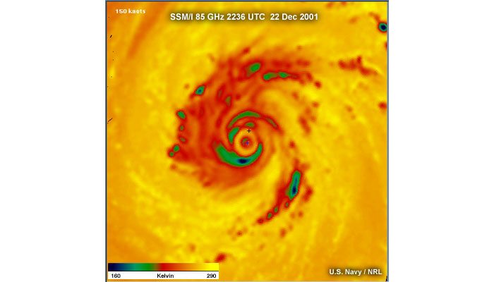
NOTE: Please use the "Page Setup" item from the "File" menu in your browser to set the orientation to "Landscape" format (11" wide by 8.5" tall) to insure the document prints correctly.
1.1 Introduction
1.2 Going Beyond Radar
1.2a Visible and Infrared Remote Sensing
1.3 SSM/I: A Revolution in Tropical Cyclone Analysis
and Forecasting
1.4 Active
Microwave Sensing
1.5 Passive Microwave Sensing
1.6 The TRMM TMI and Precipitation Radar Sensors: Tropical Cyclone Manou
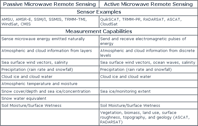
1.6a Comparing Active and Passive Microwave Sensors
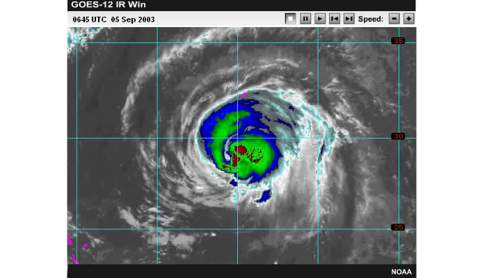
1.7 GOES IR Loop of Hurricane Fabian
1.8 Microwave “Hits” in Hurricane Fabian
1.9 Summary
2.1 Hurricane in the Southern Hemisphere:
85 GHz Color Combination
2.2 Cyclone Fay off North Coast of Australia: 89
GHz
2.3 WindSat Imagery of Hurricane Francis: 37 GHz
2.4 Tropical Cyclone Makes Landfall in India and
Pakistan: 85 GHz
2.5 Hurricane Juliette: 85 GHz
2.6 Super Typhoon Dianmu: 89 GHz
2.7 Hurricane Isabel Makes Landfall: 85 GHz
2.8 Hurricane Isabel Doppler Radar Loop
2.9 Summary
3.0 Current Passive Microwave Sensors
3.1
Introduction
3.2 Tropical Cyclone Web Pages
3.3 Conical Scanning Instruments
3.4 Passive Microwave Conical Scanning
3.5 Cross-track Passive Microwave Scanning
3.6 Cross-track Scanning AMSU vs. CMIS
3.7 AMSU-B Versus SSM/I Imagery: Super Typhoon Podul
3.8 Gaps Between AMSU-B 89 GHz Passes: Hurricane Mitch
3.9 Passive Microwave
Conical Scanning Missions
3.10 Summary
4.0 Improvements with NPOESS Conical Microwave Imager Sounder (CMIS)
4.1 NPOESS CMIS Heritage
4.2 Special Sensor Microwave Imager Sounder SSMIS
4.3 Advanced Microwave Scanning Radiometer AMSR-E
4.4 WindSat
4.5 CMIS Coverage
4.6 CMIS Products
4.7 Conical Scanning Radiometers
4.8 SSM/I and CMIS Footprint Resolutions
4.8a Graphical View of SSM/I vs. CMIS Footprints
4.9 Summary
5.0 Characteristics of Microwave Imagery
5.1 Radiative Processes at 85 GHz
in a Convective Atmosphere
5.2 Radiative Processes at 37 GHz in a Convective Atmosphere
5.3 Imagery Examples at 37 and 89 GHz: Hurricane Parma
5.4 Parallax at 85 GHz
5.5 Parallax at 37 GHz
5.6 Typhoon Jelawat at 37 GHz
5.7 Typhoon Jelawat at 85 GHz
5.8 Summary
6.0 85 to 91 GHz Imagery - Interpretation Strategies
6.1 How do I interpret a microwave
image? Hurricane Isabel
6.2 Visible Imagery of Hurricane Isabel
6.3 Color Correction: Hurricane Isabel
6.3a Storm convection or exposed ocean? Hurricane Gert
(85 GHz)
6.4 Where’s the center of Hurricane Gafilo?
IR
6.5 Where’s the center of Hurricane Gafilo?
Visible
6.6 Where’s the center of Hurricane Gafilo?
TMI 85 GHz
6.7 Summary
7.0 Multispectral Examples and Exercises
7.1 Where’s the eye of Cyclone
Fay? 89 vs. 37 GHz
7.2 Can you find the center of Tropical Storm Claudette?
7.3 Is there an eye? Hurricane Gaflio
7.4 Where’s the center of Tropical Depression
Linda?
7.5 Comparing 36/37 GHz Images: Hurricane Ketsana
7.6 Find the Center of Dianmu
7.7 Comparing SSM/I and TMI Images of Dainmu
7.8 Summary: 85-91 GHz
7.9 Summary: 37 GHz
8.0 Concentric Eyewall Characteristics
8.1 Introduction: Faxai, Guillermo,
and Juliette
8.2 Concentric Eyewall Evolution Modes: Typhoon Saomai
8.3 Concentric Eyewall Evolution Example: Super
Typhoon Winnie
8.3a Image Morphing
The use of microwave data from polar-orbiting satellites is crucial to today’s operational forecasters. This is particularly true for those with maritime forecasting responsibilities where in situ observations are sparse. This module introduces image-based techniques for analyzing tropical cyclones through case examples and conceptual models.
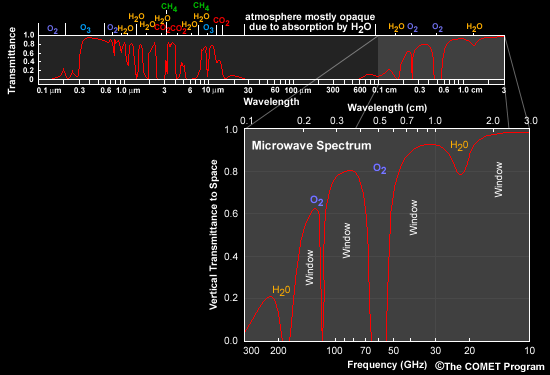
Much of the module focuses on the interpretation of clouds and precipitation patterns as seen in microwave imagery using the 37 and 85-91 GHz regions of the electromagnetic spectrum. These two spectral regions are considered important tools for tropical cyclone analysis. They reveal storm structures important for accurate storm center positioning and improved forecasts of storm motion and evolution.This module introduces forecasters to the use of microwave image products for observing and analyzing tropical cyclones. The emphasis of the module is on storm structure and techniques for improved storm positioning.
After completing the module the learner will be able to:
In order to maximize learning from this module, learners should have a working knowledge of remote sensing principles, a general knowledge of tropical cyclone structure, and a basic knowledge of meteorology.
Introductory material on polar-orbiting satellite meteorology can be found at the COMET® MetEd Website in the Satellite Meteorology program area. Specific modules that provide introductory and background information include:
Polar Satellite Products for the Operational Forecaster:
Module 1: Introduction
Module 2: Microwave
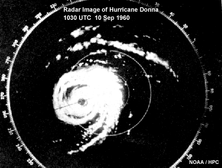
Before the advent of meteorological satellites in the 1960s, the only images seen of tropical cyclones were from ground-based weather radar. Viewers of these images marveled at the intricate structures and the symmetry of such systems. This radar image is from Hurricane Donna in 1960. Radar images are still crucial to evaluate the landfall of hurricane-force winds and torrential precipitation associated with tropical cyclones. Ground-based weather radars, however, can only detect rainbands when the storms move near or over land. By the time the radar senses the storm, it may be too late to use the information to save lives and property.
1.2a Visible and Infrared Remote Sensing
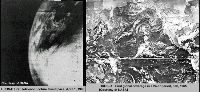
Polar-orbiting satellites were the first to send visible and infrared images, starting with the TIROS-I in 1960. Geostationary satellites provided a new level of temporal continuity beginning in 1966 with the launch of ATS-I.
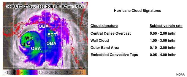
Improvements in spectral, spatial, and temporal resolution have made geostationary satellites the main tool for measuring tropical cyclone intensity. Microwave imagers and radiometers enhance this capability by sensing storm structure and intensity through cirrus shields that hamper visible and infrared imagers and sounders. Less is said about visible and infrared sensor systems as they are covered in other materials. Please see the Resources page for more information.
1.3 SSM/I: A Revolution in Tropical Cyclone Analysis and Forecasting
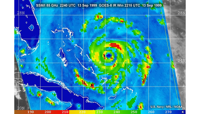
All that changed in 1987 when the F-8 satellite containing the
first Special Sensor Microwave Imager (SSM/I) was launched by the Defense Meteorological
Satellite Program (DMSP) and it began to transmit spectacular images of tropical
cyclones over the open ocean. Lacking the high temporal or spatial resolution
of ground radar, SSM/I was sometimes called a “poor man’s radar.”
Actually, SSM/I has different strengths compared to ground radar. It can cover
vastly more territory, especially over ocean areas. It can greatly assist warning
efforts when storms are approaching land, but are still too far away to be imaged
from shore-based radar. It can show in detail the previously unobserved processes
of formation, intensification and decay, and landfall. It can see low-level
structure missed by other weather satellite sensors. Perhaps most importantly,
it can be used to fix the center of these systems to assist forecasting. Better
center fixes also mean better warnings to ships and coastal populations and
better initialization of numerical models.
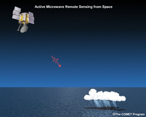
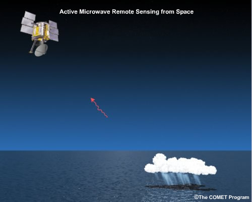
Active microwave radiometers have an onboard power supply used to send periodic pulses of energy toward the earth. Weather radars located on the earth’s surface, such as Doppler, work in a similar way.
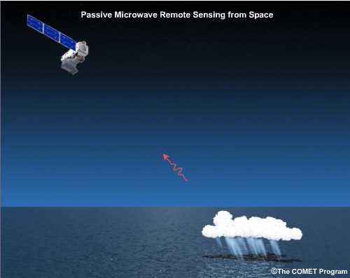
Passive microwave radiometers, on the other hand, send no pulses out toward the earth. Instead, the sensor receives radiation naturally emitted from the earth/atmosphere system, including from precipitation. The passive instrument, sensing existing microwave radiation, has the advantage of requiring much less ongoing power than an active system. This strategy is a relatively inexpensive way to collect huge amounts of information about tropical cyclones over oceans. We will be addressing passive microwave radiometry in this module.
1.6 The TRMM TMI and Precipitation Radar Sensors: Tropical Cyclone Manou
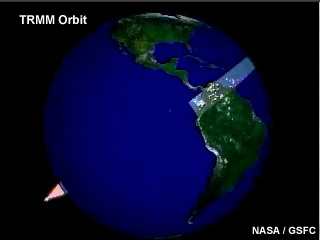
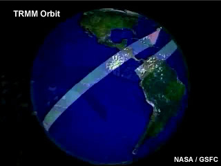
The TRMM satellite has both active and passive microwave sensors on board. The TRMM precipitation radar (PR) is the active sensor and gives precise information about rain rate. But for fixing tropical cyclones, the TRMM PR is unnecessary. The TMI, the passive sensor, gives us more than adequate information, and it provides more spatial coverage than the TRMM PR.
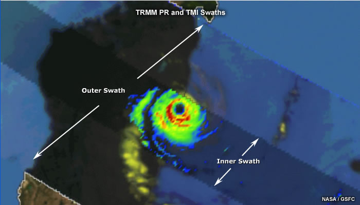
In this view, we see the orbital swath of TRMM cutting across Madagascar. The outermost swath represents the scanning path of the TMI, which is able to detect precipitating ice particles in the top of Manou's outer rainbands. The innermost swath shows rain intensity in the storm core as measured by the PR.
1.6a Comparing Active and Passive Microwave Sensors
1.7 GOES IR Image of Hurricane Fabian
Most reconnaissance aircraft penetrations are performed in high-priority
Atlantic storms. Elsewhere, forecasters need to locate the center of the storm
using satellite imagery alone. But if no eye is readily apparent, the analyst’s
job becomes more complicated.
Here is an IR loop of Hurricane Fabian over a 24-hour period. Although the storm
has an intensity of 105 knots, there are only occasional hints of an eye in
this imagery. For storm trackers, using only infrared images like these makes
determining a center of circulation a daunting proposition
1.8 Microwave “Hits” in Hurricane Fabian
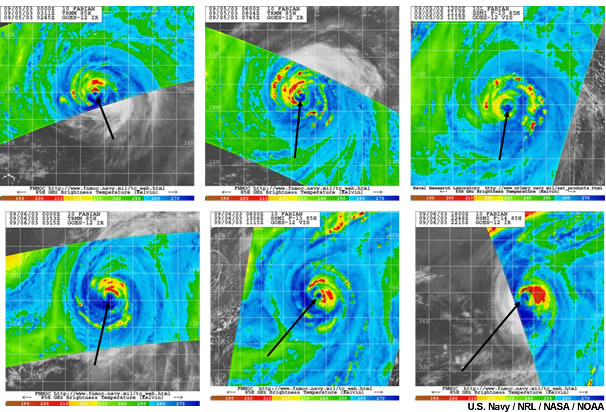
Now look at the SSM/I and TMI passes available during the same period. Each one shows an easier-to-find center than seen in the corresponding infrared imagery. Any one of these could be used to determine a center fix. In the NPOESS era such images will be available within 30 minutes of overpass time, accelerating timely support to forecasters.
2.1 Hurricane in the Southern Hemisphere: 85 GHz Color Combination
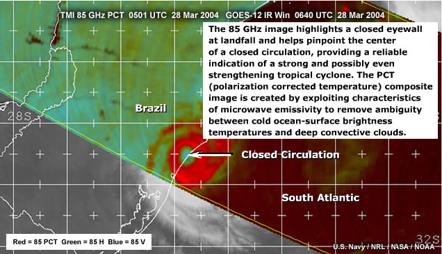
Let’s take a tour around the globe to see how passive
microwave sensors view tropical cyclones. At this point don’t worry about
understanding everything you see. We will go into more detail later.
Passive microwave imagery, such as this 85-GHz image from the NASA Tropical
Rainfall Measuring Mission (TRMM) Microwave Imager (TMI), helped confirm the
existence of a hurricane in the South Atlantic in March 2004. Prior to this
storm, many forecasters had believed that hurricanes did not occur in this ocean
basin. The storm had top winds estimated at 85 miles per hour before landfall.
The 85-GHz image highlights a closed eye wall at landfall and helps pinpoint
the center of a closed circulation, providing a reliable indication of a strong
and possibly even strengthening tropical cyclone.
2.2 Cyclone Fay off North Coast of Australia: 89 GHz
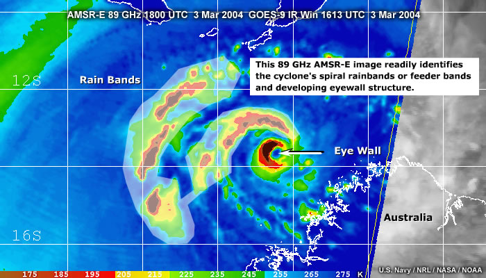
Let’s move to the North Australian coast where these
storms are called cyclones. Notice the clockwise circulation, as the storm is
in the Southern Hemisphere. This is Cyclone Fay in March 2004, imaged by the
Advanced Microwave Scanning Radiometer (AMSR-E) instrument on the Earth Observing
System (EOS) Aqua satellite. This 89 GHz AMSR-E image readily identifies the
cyclone's spiral rainbands or feeder bands
and developing eyewall structure.
2.3 WindSat Imagery of Hurricane Francis: 37 GHz
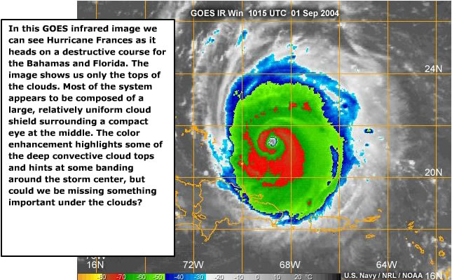
In this GOES infrared image we can see Hurricane Frances as it heads on a destructive course toward the Bahamas and Florida. The image shows us only the tops of the clouds. Most of the system appears to be composed of a large, relatively uniform cloud shield surrounding a compact eye at the middle. The color enhancement highlights some of the deep convective cloud tops and hints at some banding around the storm center, but could we be missing something important under the clouds?
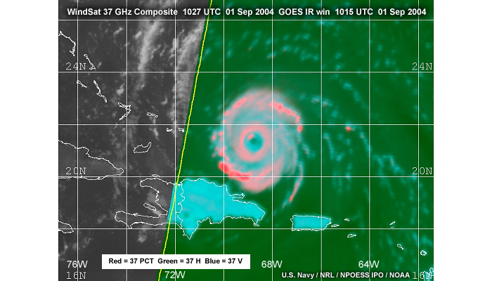
Now let's look at the WindSat 36 GHz color product. We can
see a tiny green dot in the middle representing the cloud-free eye. Surrounding
the eye, a fierce eyewall in pink is associated with torrential rain and hurricane-force
winds at the surface. Toward the periphery lies another concentric series of
rainbands containing severe weather. These secondary bands, not as apparent
in the infrared image, give forecasters vital information about the destructive
power of the storm.
The WindSat microwave imager is very similar to the CMIS sensor planned for
the NPOESS satellites. We'll say more about it later.
2.4 Tropical Cyclone Makes Landfall in India and Pakistan: 85 GHz
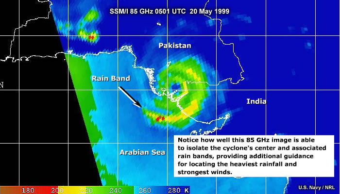
Here is an intense tropical cyclone moving into India and Pakistan from the Arabian Sea. This is an SSM/I pass from Tropical Cyclone 02A from 1999. This kind of imagery is invaluable as a basis for early warnings to coastal populations. Notice how well this 85 GHz image is able to isolate the cyclone's center and associated rain bands, providing additional guidance for locating the heaviest rainfall and strongest winds.
2.5 Hurricane Juliette: 85 GHz
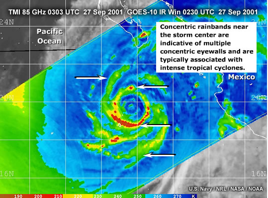
Let’s move to the eastern Pacific and view an 85 GHz image of Hurricane Juliette from the TMI. Notice the multiple rainbands. We will say more about this later. In this image greens, yellows, and reds indicate heavy precipitation.
2.6 Super
Typhoon Dianmu: 89 GHz
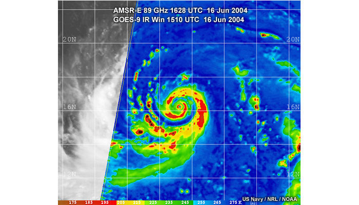
Sometimes the most powerful storms have miniscule eyes. Super Typhoon Dianmu in the western North Pacific, with maximum winds estimated at 155 knots, is an example. This was a Category 5 storm, the most intense designation.
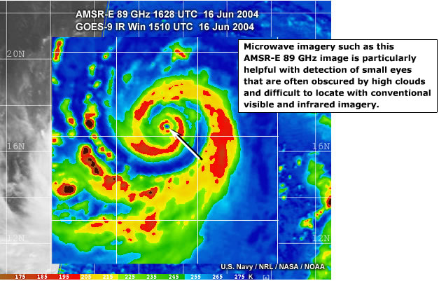
Microwave imagery such as this AMSR-E 89 GHz image is particularly helpful with detection of small eyes that are often obscured by high clouds and difficult to locate with conventional visible and infrared imagery.
2.7 Hurricane Isabel Makes Landfall: 85 GHz
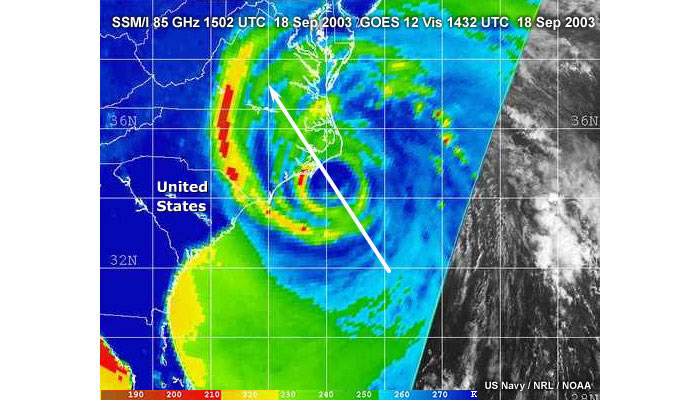
Finally, let’s look at Hurricane Isabel moving ashore on the East Coast of the United States.
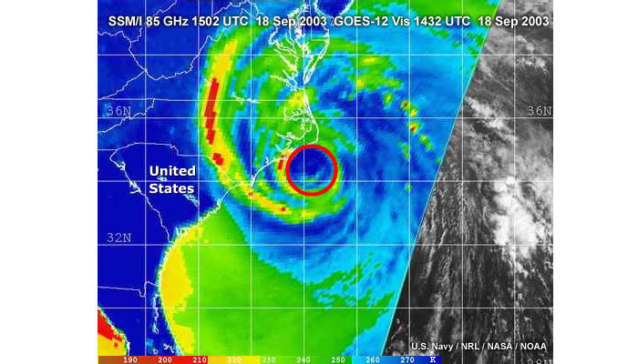
The eye is quite large in this SSM/I image, clearly showing the intense rainbands outlined in yellow and red.
2.8 Hurricane Isabel Doppler Radar
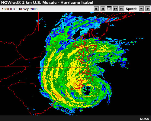
Since Isabel is near the coast, we see a similar pattern in the ground radar. This radar loop confirms the large eye and the position of the rainbands shown by the SSM/I.
3.0 Current Passive Microwave Sensors
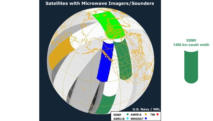
Let’s learn a little about the satellite instruments and orbits that produce this imagery. Passive microwave swaths are relatively narrow, but the large number of sensors compensates for this limitation somewhat. Here are the sensors flying in 2004. The SSM/I sensors with a width of 1400 km appear in green. They come one right after the other over a given location in the morning or the evening.
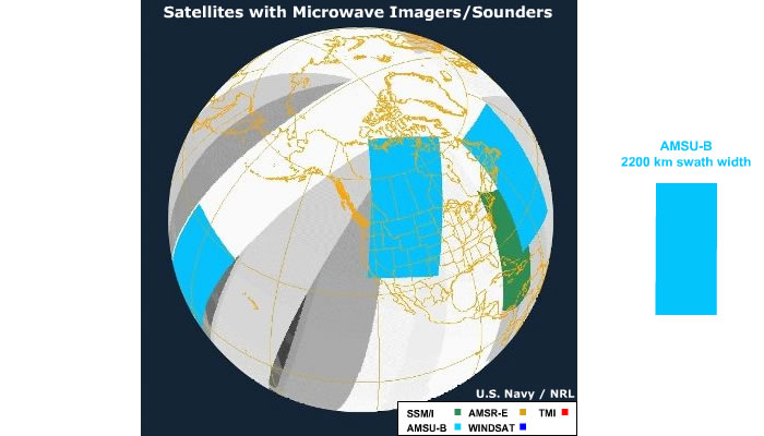
AMSU-B swaths, 2200 km wide, appear in light blue.
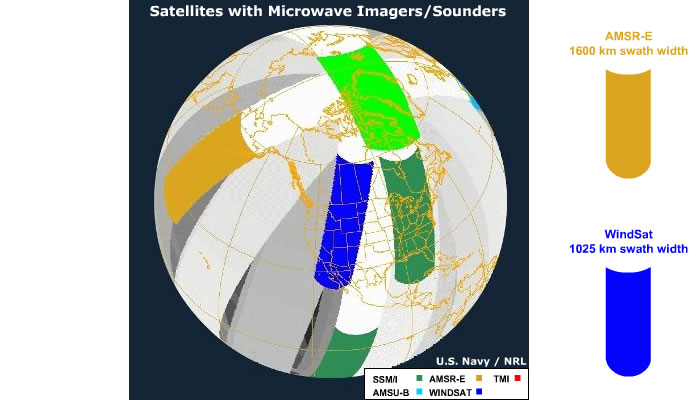
Next we see two research satellites that have been successfully pressed into service for operations: the AMSR-E in tan, 1600 km wide, and WindSat flying aboard the Coriolis satellite in dark blue, with a 1025 km swath width. White indicates that a region was recently covered, fading to darker and darker gray as the coverage ages. Notice, however, that no region stays dark gray for long. Fresh data arrives from the large number of new orbits.
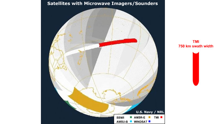
The poles have the most overlapping coverage, but even in the Tropics, our area of interest, data are refreshed frequently. Finally, we see the near-equatorial orbit of the TMI in red with a 750 km swath. It was put into orbit originally to measure precipitation in the Tropics, but has become one the finest satellite hurricane hunters ever.
3.2 Tropical Cyclone Web Pages
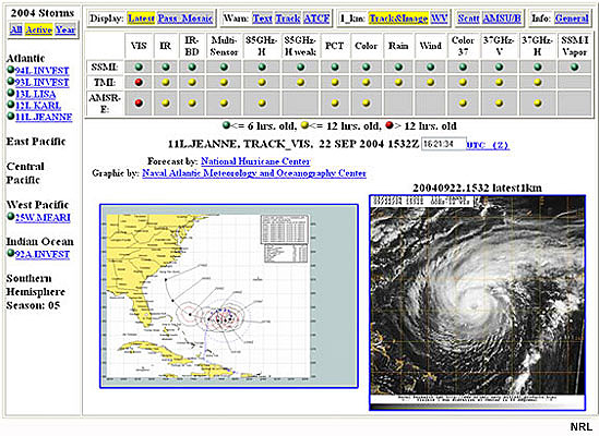
Fortunately, Web applications can consolidate the information from all these satellite passes, allowing easy monitoring of tropical cyclones by users. The NRL Monterey Tropical Cyclone Web Page provides multisensor information on each active tropical system around the world. FNMOC maintains a similar site.

These sites combine polar-orbiting microwave imagery with geostationary visible and infrared imagery to provide users with enhanced analysis capabilities. Many of the examples shown in this module were taken directly from products from these Web applications.
3.3 Conical Scanning Instruments
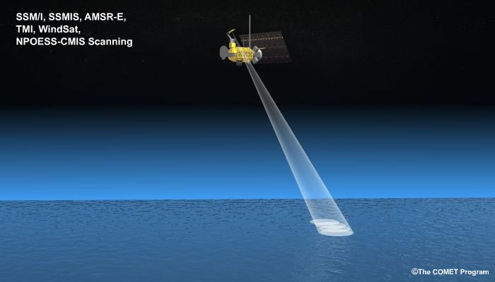
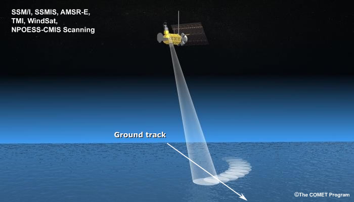
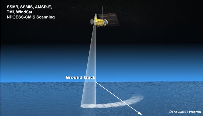
Let’s look at the SSM/I scan pattern. The NPOESS Conical Microwave Imager Sounder (CMIS) will operate in the same way. The antenna rotates as the satellite moves in its orbit, but only the forward-portion of the swath is used for data. An advantage of conical scanning is that all the footprints are the same size, eliminating distortion at the edge of passes.
3.4 Passive Microwave Conical Scanning
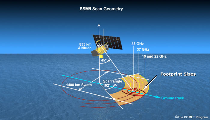
Here’s a schematic of the S
SM/I conical scan with a 1400-km wide swath. Notice how the satellite at 833 km above the earth always looks forward at a fixed angle. This has important implications for parallax error for tropical cyclone monitoring. The concentric ovals represent footprint sizes of different frequencies.
3.5 Cross-track Passive Microwave Scanning
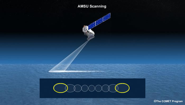
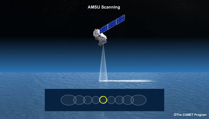
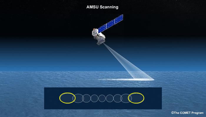
There are other instruments that view tropical cyclones at passive microwave frequencies. Here is an animation of the scan pattern used by the Advanced Microwave Sounding Unit (AMSU-B) aboard the NOAA satellites. This instrument was intended as a sounder, but it can also be used for imaging. This is a cross-track scanner, so the scan angle varies as the instrument points away from nadir. Thus, the footprints get bigger at the edge of an orbit swath, a limitation we will discuss.
3.6 Cross-track Scanning AMSU vs. CMIS
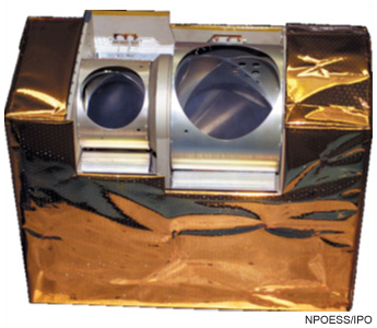
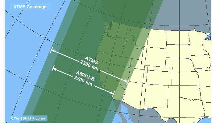
Cross-track microwave radiometers have relatively poor spatial resolution, but make up for it with broad swaths. Consider the Advanced Technology Microwave Sounder instrument (ATMS), which will fly first on the NPOESS Preparatory Project (NPP) satellite. The ATMS 89-GHz spatial resolution will be the same as the current AMSU-B, but the swath will increase to 2300 km.
3.7 AMSU-B Versus SSM/I Imagery: Super Typhoon Podul
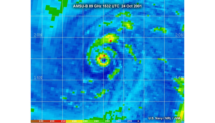
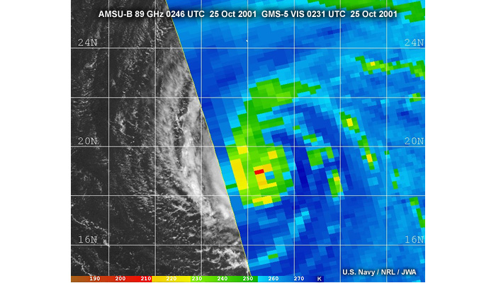
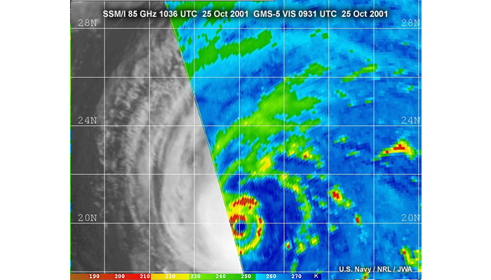
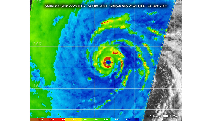
To illustrate the differences between conical and cross-track imaging, let’s compare SSM/I and AMSU-B images, all taken at about the same time over Super Typhoon Podul. The 89 GHz image from AMSU-B looks fine near nadir (the image on the left) but degrades toward the edge of scan (as shown on the right) because of pixel enlargement there. This can make detection of the storm center difficult. The conically-scanning SSM/I doesn’t have this drawback. The typhoon structure is as sharp near the edge of scan (right) as it is closer to the center (left).
3.8 Gaps Between AMSU-B 89 GHz Passes: Hurricane Mitch
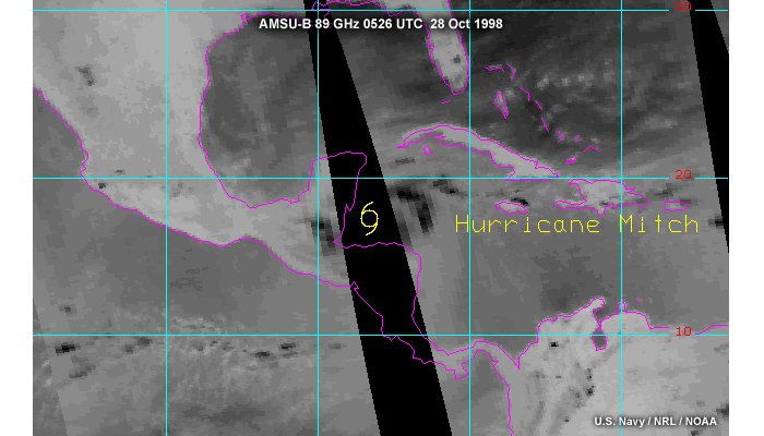
Here we consider the coverage by a single polar-orbiting satellite.
Gaps between successive passes shown for the AMSU-B will be eliminated for NPOESS
ATMS. The AMSU-B swaths shown here are already quite wide compared to SSM/I,
but there is still a gap between orbits at low latitudes. Look what happens
to Hurricane Mitch in this example. The ATMS will have no gaps between orbits,
and thus will always image a storm twice a day.
3.9 Passive Microwave Conical Scanning Missions
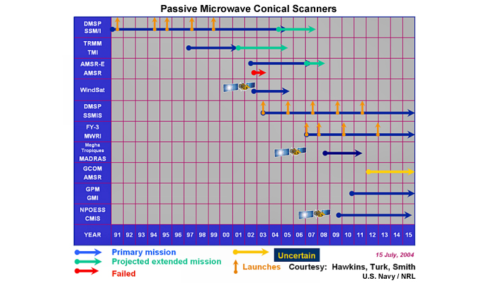
The first five rows here summarize recent passive microwave conical scanners. The workhorse sensor, the SSM/I, is nearing the end of its planned lifetime. The SSM/I series is being replaced by the DMSP SSMIS with more channels and a wider swath.
TMI and Aqua AMSR-E are research missions. We mention them here because they serve as demonstrations for the NPOESS CMIS mission. TMI serves as a precipitation measurement sensor. AMSR-E orbits on the NASA Aqua satellite to study the global water cycle. WindSat is a Navy satellite sensor primarily intended to measure surface wind speed and direction over the ocean, but will be useful as an imager for tropical cyclones as well. Note that CMIS will not fly on the NPOESS NPP, but will wait for NPOESS launches. The other satellite missions shown are research and international systems that may be used for operational monitoring of tropical cyclones.
4.0 Improvements with
NPOESS Conical Microwave
Imager Sounder (CMIS)
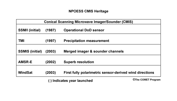
CMIS builds on a number of passive microwave sensors over the last 25 years. We have seen images from several of the most important heritage sensors, but now let’s take a close look at the instruments themselves and their capabilities.
4.2 Special Sensor Microwave Imager/Sounder SSMIS
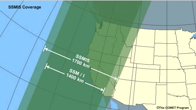
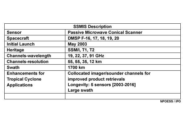
The SSMIS was designed as the SSM/I follow-on and is now continuing
the previous sensor’s mission. First flown on DMSP F16, SSMIS has a 1700-km
wide conical swath, compared to just 1400 km for SSM/I. As of 2004 there were
four additional SSMIS sensors awaiting launch.
The SSMIS combines imager and sounder channels in the same view, simplifying
combined algorithm development and implementation. We only list the imager channels
here. The sounder channels will also serve an important purpose providing estimates
of tropical cyclone intensity.
4.3 Advanced Microwave Scanning Radiometer AMSR-E
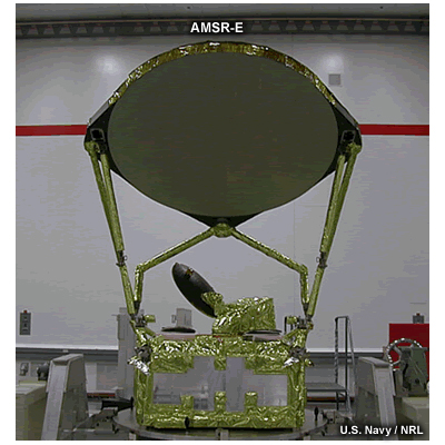
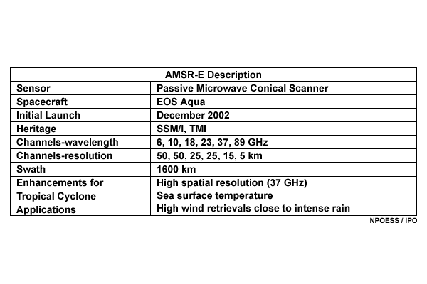
The AMSR-E onboard the NASA EOS Aqua spacecraft is a Research and Development sensor with superb spatial resolution. It includes important low frequency channels at 6 and 10 GHz needed for surface wind speed and sea surface temperatures. With a 1.6 meter diameter, the AMSR-E antenna is much larger than the ones used for SSM/I and TMI.
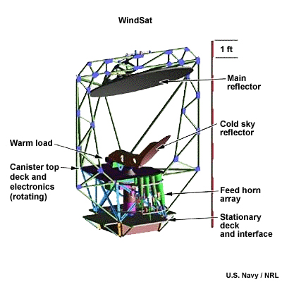
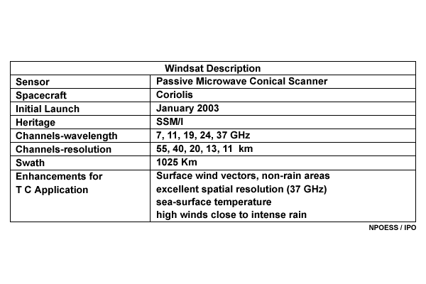
WindSat is a U.S. Navy sensor designed to retrieve both surface wind and speed, via polarimetric radiometry. It serves as a proof of concept to anticipate CMIS on NPOESS. WindSat can also contribute valuable imagery for the analysis of tropical cyclones
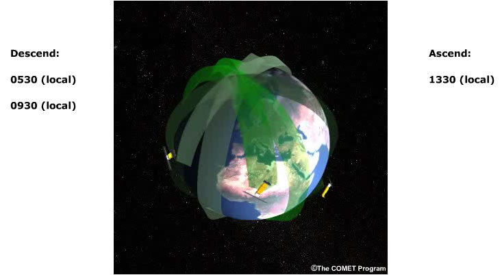
CMIS will travel on NPOESS in the three-orbit configuration. One will descend at 0530 local time, another descending at 0930 local time. The third and final sensor will ascend at 1330 local time. Together these three satellites will provide superior coverage accuracy, but they will not be alone in the monitoring mission. Additional microwave sensors—U.S. and international—will provide additional coverage. CMIS represents a new era in storm monitoring, supplying data to forecasters in a matter of minutes after overpass, far faster than current polar-orbiting satellite systems.
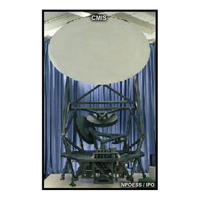
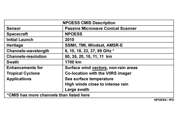
Like WindSat, NPOESS CMIS will retrieve the complete surface wind vector via polarimetric radiometry. Like TMI, it will provide very high-resolution images with a wider 1700 km swath. Like AMSR-E, it will be capable of calibrated, high-resolution geophysical products, like sea surface temperature. Advantageously, the CMIS data will be synergistically combined with data from the NPOESS VIIRS visible/infrared sensor for more accurate and complete data.
4.7 CMIS Antenna and Product Improvement
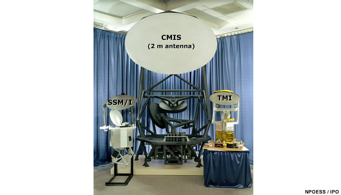
A key to the success of CMIS will be its large antenna, 2 meters in diameter. Compare this antenna to those of the TMI and SSM/I. The larger the antenna, the finer the spatial resolution of the data. Fine resolution will in turn lead to huge increases in the quality of images and products. Note that the tropical cyclone mission is only a relatively small part of the mission of CMIS. Compared to SSM/I, CMIS is both an imager and a sounder. Thus, it will provide a powerful data stream for assimilation into numerical models.
4.8 SSM/I and CMIS Footprint Resolutions
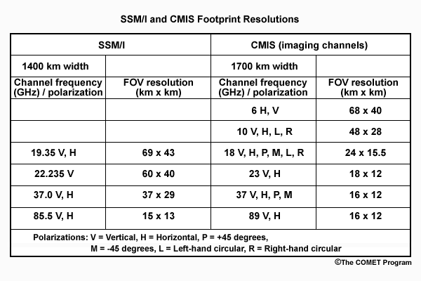
Here we list only the CMIS channels most relevant to the fixing of tropical cyclones. Compared to SSM/I, CMIS will provide greatly improved effective field of views or spatial resolution for most channels. Better than a factor of two improvement will be realized for 18, 23, and 37 GHz channels when compared to the corresponding channels on the SSM/I sensor.
4.8a Graphical View of SSM/I vs. CMIS Footprints
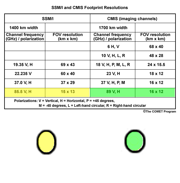
The highest CMIS frequency, the CMIS 89 GHz channel, has a footprint comparably sized to the SSM/I 85 GHz. However, improved engineering on CMIS should still lead to a significant improvement in 89 GHz CMIS product quality compared to that of the SSM/I.
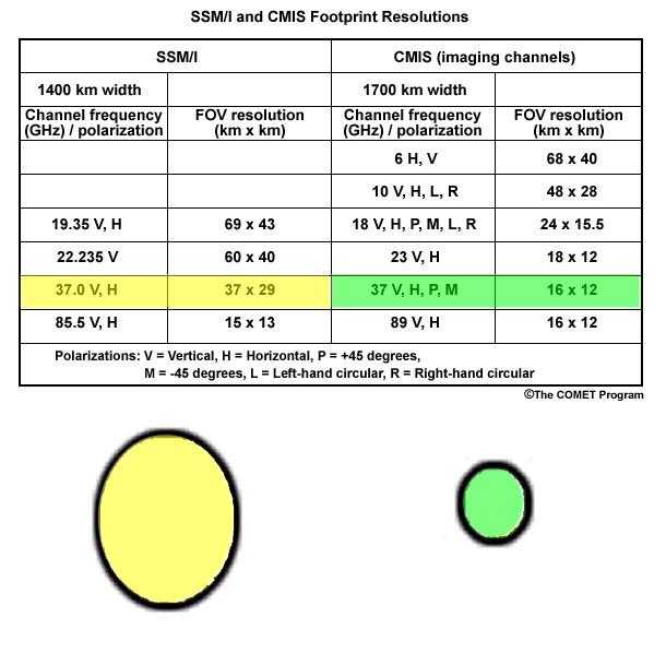
A key improvement is the 37 GHz channel. Very important for tropical cyclone monitoring, the channel is too coarse for effective monitoring using the SSM/I. In the CMIS era, its much smaller size will support much more detailed images, similar to what we saw earlier with AMSR-E and TMI.
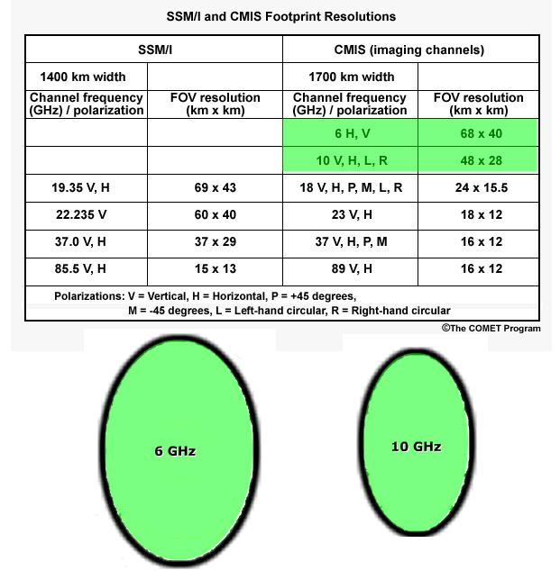
Applications for tropical cyclones will also be found for the lower frequencies, especially at 6 and 10 GHz, which should, for example, enable better retrieval of winds in conditions of heavy clouds and rain.
5.0 Characteristics of Microwave Imagery
5.1 Radiative Processes at 85 GHz in a Convective Atmosphere
We will look at two main passive microwave channels used for storm analysis, one from about 85 to 91 GHz and another near 37 GHz. The exact frequencies vary depending on the sensor.
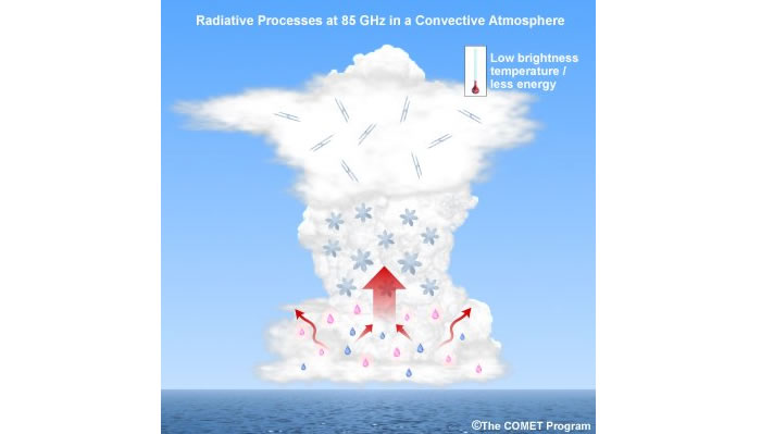
In the 85 GHz region, radiation leaves the ocean, but it doesn't
get very far before either getting absorbed and re-emitted by cloud droplets
and raindrops in the cloud system or scattered by these droplets out of the
satellite's field of view.
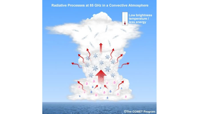
Much of the remaining energy is further scattered by large precipitating ice
particles above the freezing level. Non-precipitating cirrus near the top of
the storm has little effect on radiation at this wavelength.
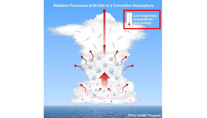
But scattering by the large ice particles below has already seriously depleted the radiation stream, and only a small number of photons leave cloud top. This leads to very low satellite brightness temperatures in these areas.
5.2 Radiative Processes at 37 GHz in a Convective Atmosphere
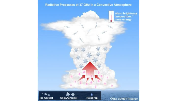
In the 37 GHz region, radiation rising from the ocean is absorbed by cloud and rain water.
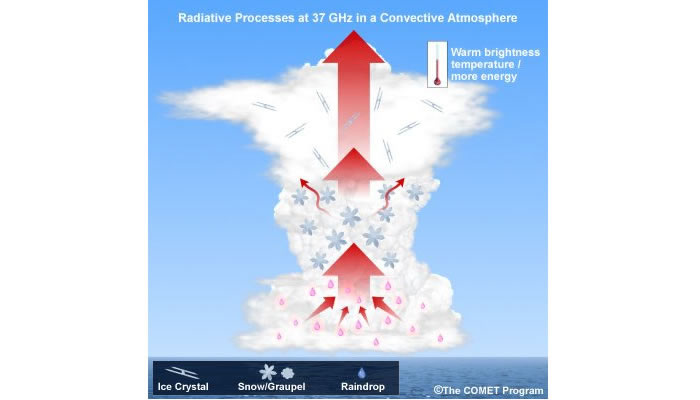
The radiation emitted from the cloud and rain water upwells further and undergoes only minor scattering by precipitation-sized ice particles. High, non-precipitating cirrus has little effect on microwave radiation at this wavelength, so that abundant radiation reaches the satellite, resulting in high brightness temperatures.
5.3 Imagery Examples at 37 and 89 GHz: Hurricane Parma
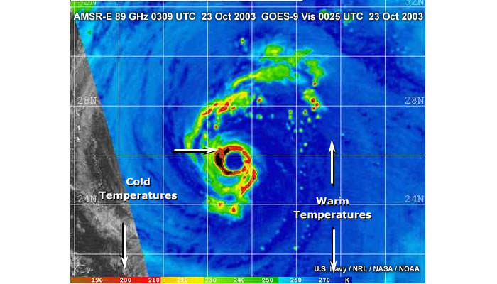
If we look at an AMSR-E 89 GHz image, we see cold temperatures of deep convection in red against a warmer ocean background in blue. Note that we are showing this image using a reversed color table. Blues show warm temperatures, and reds show cold temperatures.
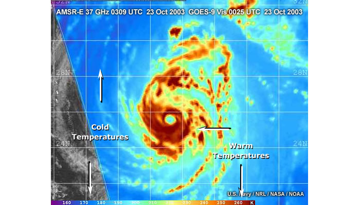
The corresponding 37 GHz image is shown with a more standard color table, meaning red is warm and blue is cold. In this channel we see the warm temperatures of rain at low levels as red against a cooler ocean background in blue. We're looking at precipitation in both instances, but the primary mechanism for sensing the precipitation is different.
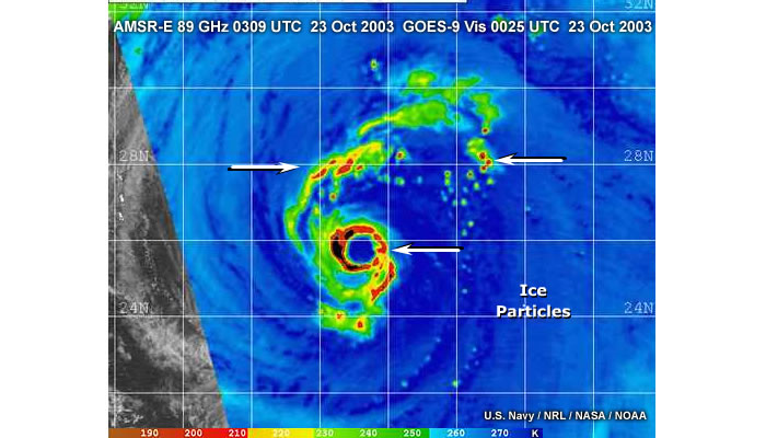
The 89 GHz channel shows it to us as ice precipitation high in the storm system;
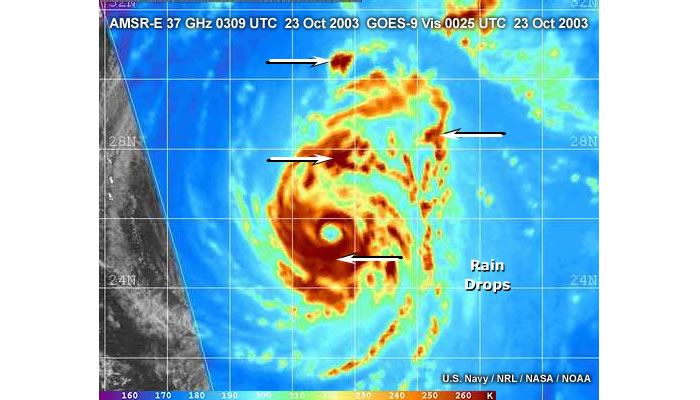
the 37 GHz channel shows us the precipitation once it becomes more liquid below the freezing level. Images based on frequencies at or near 85 GHz have become the standard for interpretation because they have higher spatial resolution and show deep, cold convection well. However, images from the 37-GHz channel have a number of advantages which we will discuss.
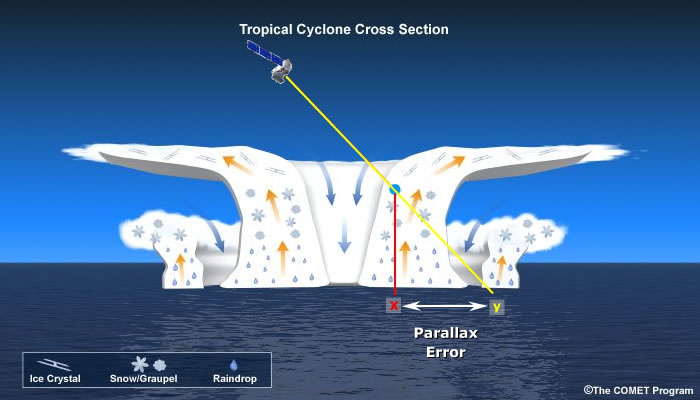
The parallax viewing effect changes the positioning of the centers of tropical cyclones on images. The diagram here isn't drawn to scale but gives an idea of this parallax offset, which has different magnitudes for the two main imaging frequencies. At 85 GHz, the satellite detects precipitation as ice particles high in the cloud system, above point X on the surface of the earth. But because of the slant viewing angle, the satellite-derived position is displaced to point Y. The distance between X and Y is called the parallax error.
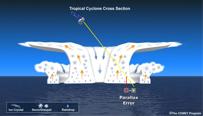
The raindrops sensed at 37 GHz, are much lower in the cloud as shown in the conceptual model. The displacement due to viewing geometry still occurs, but is less, so the parallax error is less.
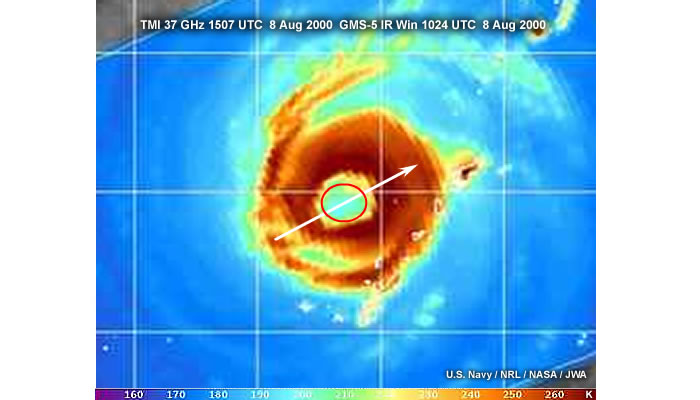
Here is a TMI 37 GHz image of a Western Pacific typhoon where
the browns and oranges indicate heavy clouds or rain. The arrow indicates the
direction of the parallax projected onto the image. But the parallax displacement
is small. Thus, the center of the image eye is approximately the true geographic
center of the storm.
The red circle marks the eye.
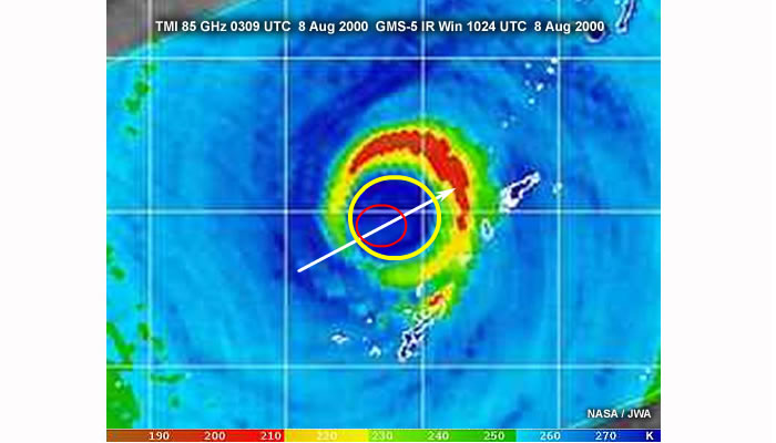
Now let's look at the corresponding 85 GHz image of this storm with the same fix position we applied to the 37 GHz image. The displacement occurs because the parallax error is so much greater at 85 GHz compared with 37 GHz.
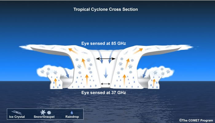
Notice the slight spreading of the eye into an oval in the 85 GHz image. The eye looks bigger at 85 GHz because the 85 GHz eye represents conditions higher in the storm where the eye is larger than near the surface. Parallax error at 85 GHz can range from about 10 to 20 km from the true position. Parallax error at 37 GHz is probably 5 km or less.
6.0 85 to 91 GHz Imagery - Interpretation Strategies
6.1 How do I interpret a microwave image? Hurricane Isabel
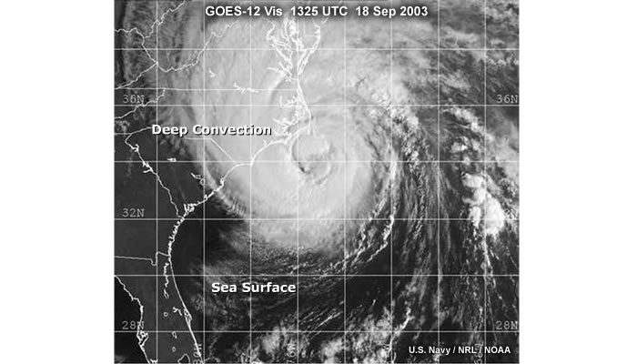
Let's examine a typical SSM/I 85 GHz image of Hurricane Isabel.
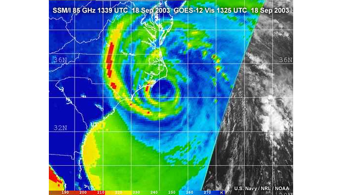
First, cloud-free land will always appear warm compared to ocean, because land is almost a blackbody radiating surface at this frequency and emits energy efficiently toward the satellite. Thus, in this SSM/I 85 GHz image, the United States is blue, indicating temperatures higher than 270 Kelvin.
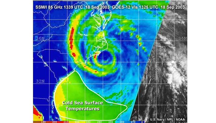
Second, the ocean is cold when not covered by heavy clouds, water vapor, or precipitation. Here the cold ocean regions are shown in red, yellow, and green, having temperatures from about 210 to 250 Kelvins. These cold temperatures do not mean that the ocean is physically cold. Rather it is "radiometrically cold" at this frequency because the ocean has low microwave emissivity, meaning that is does not radiate efficiently toward the satellite.
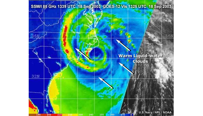
Dense water vapor and especially low cloud bands, shown here in blue, are warm. Physically, these clouds are at a lower temperature than the sea surface, but at 85 GHz, they appear about 20 to 30 degrees Celcius warmer.
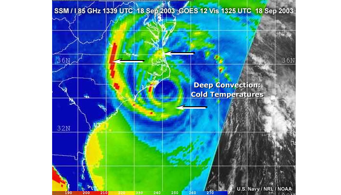
Finally, convective precipitation, shown in the image as greens, yellows, and reds, is cold. These low temperatures are caused by precipitation-sized ice particles high in the cloud system that scatter microwave energy at 85 GHz away from the view of the satellite. The start of the green color in this example denotes temperatures low enough to indicate significant precipitation.
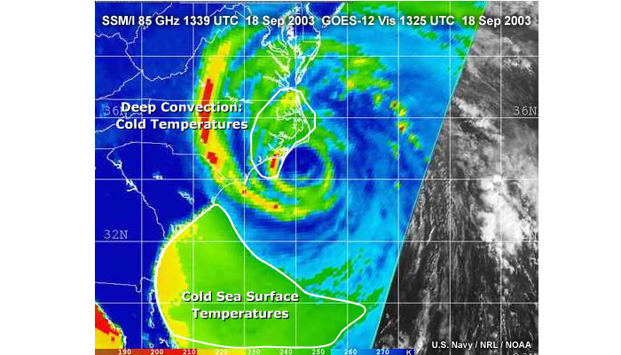
Often, the cold ocean has the same temperature as deep convection and distinguishing between the two is difficult. For example, it is hard to distinguish the cold temperatures of a convective rainband over North Carolina from the cold temperatures of the ocean capped by dry air off South Carolina, Georgia, and Florida.
6.2 Visible Imagery of Hurricane Isabel
Here’s an early morning visible image of Claudette as
a Tropical Storm with winds about 55 knots. Let’s say you’re the
analyst charged with fixing the center. People along the coast are starting
to worry, and a good forecast depends on finding the center correctly. Storms
at 55 knots often have eyes: Can you locate it?
Answer: Cirrus covers the storm and obscures our view of the storm interior.
Thus, you do not get much information from this image.
6.3 Color Correction: Hurricane Isabel
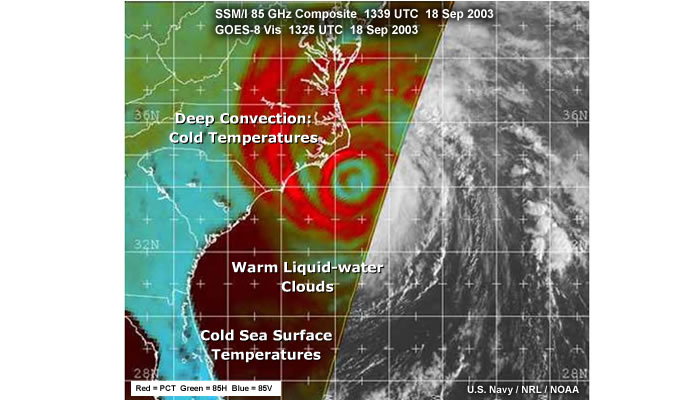
A popular 85 GHz color enhancement is another way to eliminate the confusion between radiometrically cold ocean and deep convection. Here, deep convection is red; cloud water over ocean appears as cyan; ocean regions free of low-level clouds are dark brown. No ambiguity appears between the ocean surface and convective precipitation. This enhancement is available from the Fleet Numerical Meteorology and Oceanography Center (FNMOC) and the Naval Research Laboratory (NRL).
6.3a Storm convection or exposed ocean? Hurricane Gert (85 GHz)
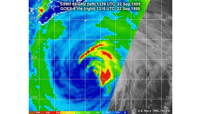
Here’s another example of potential ambiguity in an 85-GHz image of Hurricane Gert, south of Nova Scotia. This raw 85-GHz image is hard to interpret. Where does the storm convection stop and the exposed sea surface begin? Without correction, it’s hard to know. Observers can make critical mistakes if they misinterpret images like this one.
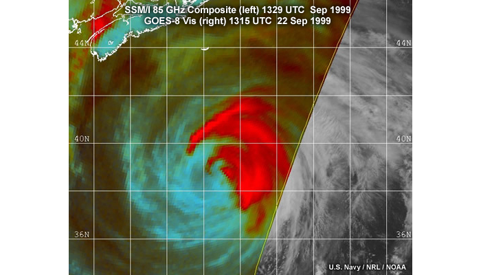
The color correction makes image interpretation easier. Red indicates deep convection, now easily distinguished from a low-level cloud circulation shown in cyan. The precipitation-free sea surface now appears dark brown and will not be confused with storm convection.
6.4 Where’s the center of Hurricane Gafilo? IR
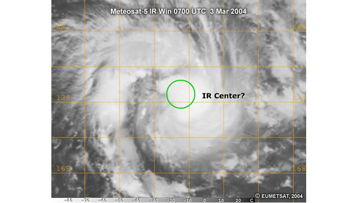
Here's another example of center positioning when cirrus obscures the storm scene. Using a standard infrared image from Meteosat, one might chose the center here for Gafilo.
6.5 Where’s the center of Hurricane Gafilo? Visible
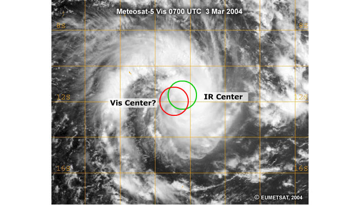
But if we look at the Meteosat visible image, our perspective changes and the red circle is perhaps the best estimate of storm center. Visible images are often better than infrared images in detecting storm centers due to higher spatial resolution. Plus, cirrus obscuration is less of a factor at visible wavelengths.
6.6 Where’s the center of Hurricane Gafilo? TMI 85 GHz
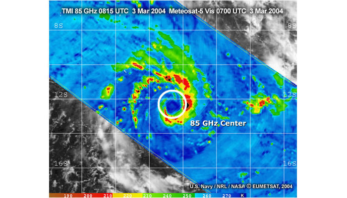
The TRMM TMI takes the guesswork out of finding the center, as we see in this 85 GHz image of the same storm scene. Cirrus is completely transparent, so the sensor sees to the center below.
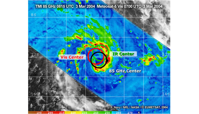
Here are all our fixes on the TMI image. Look how wrong we would
have been had we relied on visible and infrared center fixes.
At 85 GHz:
7.0 Multispectral Examples and Exercises
7.1 Where’s the eye of Cyclone Fay? 89 vs. 37 GHz
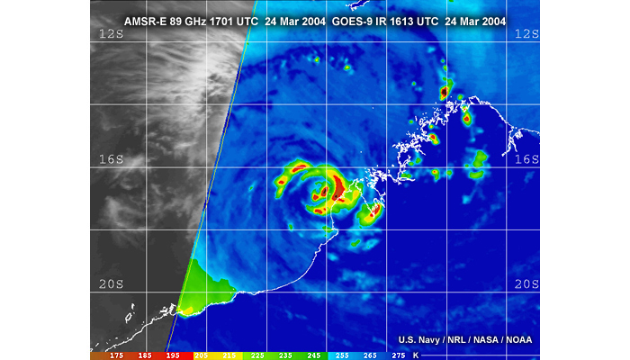
Images using the 37 GHz channel can sometimes show low-level storm circulations that are missed at 89 GHz. For example, this AMSR-E 89 GHz image shows no definite eye associated with Cyclone Fay off the northern coast of Australia.
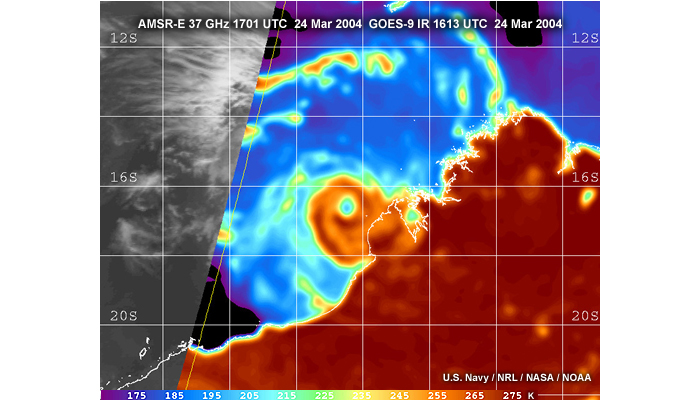
But the 37 GHz image shows the eye perfectly. This frequency is sensitive to liquid water variations in the core of storms, enabling forecasters responsible for storm fixing to pinpoint the storm’s center. Here, the red shades indicate warming due to raindrops in the storm, while the blue shades indicate cooling in the eye due to the absence of raindrops.
7.2 Can you find the center of Tropical Storm Claudette?
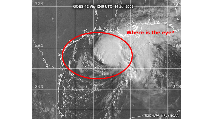
Here’s an early morning visible image of Claudette as
a Tropical Storm with winds about 55 knots. Let’s say you’re the
analyst charged with fixing the center. People along the coast are starting
to worry, and a good forecast depends on finding the center correctly. Storms
at 55 knots often have eyes: Can you locate it?
Answer: Cirrus covers the storm and obscures our view of the storm interior.
Thus, you do not get much information from this image.
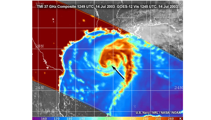
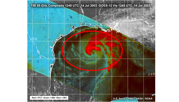
The 85 GHz color enhancement from TMI gives a better view of the storm, showing precipitation in red and other cloud bands in cyan over the Gulf, but it is still hard to identify the eye.
The 37 GHz image of the same scene shows a closed eye and gives you the center fix you want.
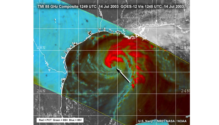
But sometimes 85 GHz imagery provides the information necessary for fixing the center. It is best to look at images at both frequencies in difficult cases.
7.3 Hurricane Gafilo: Is there an eye?
Sometimes false eyes appear on 37 GHz images when especially strong convection mimics an eye signature.
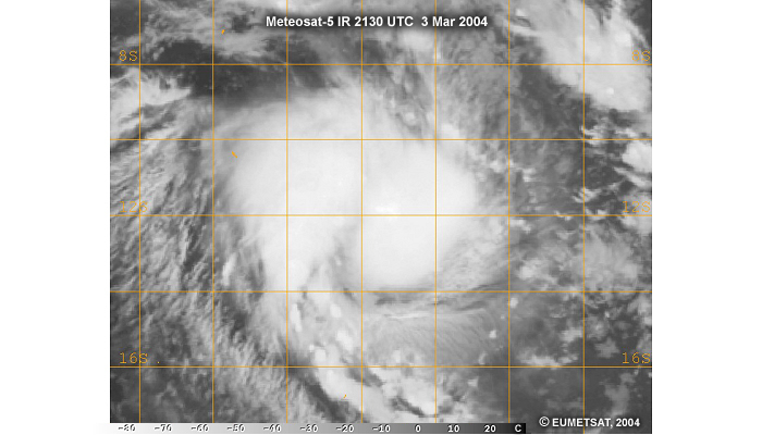
In this case the infrared image shows no trace of an eye, but an eye-like feature appears in a reasonable place on the AMSR-E 37-GHz image. Could this be the center?
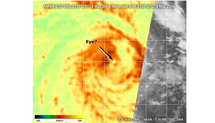
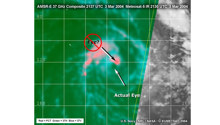
A 37 GHz color combination shows that the suspected eye is really intense convection,
colored pink in this enhancement. The real eye is not far away from our original
guess. When in doubt, forecasters can use this enhancement, which is similar
to the 85 GHz color enhancement discussed earlier, to help eliminate false eye
detections.
7.4 Where’s the center of Tropical Depression Linda?
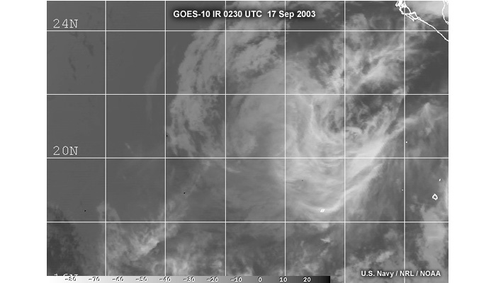
Here’s a nighttime GOES infrared shot of tropical depression Linda dissipating off Mexico. It shows a mass of disorganized cirrus, indicating a vertically sheared system. Can you find a center? Not easily. In the IR-Window channel, the cirrus is hiding our view.
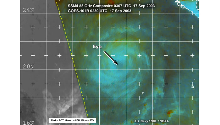
The 85 GHz frequency, however, is not sensitive to cirrus aloft. It sees through to the low-level center as shown in this SSM/I 85 GHz color combination image. Most of the convection has dissipated due to shear. However, these low-level circulations can persist for days and even regenerate into more intense storms.
7.5 Comparing 36/37 GHz Images: Hurricane Ketsana
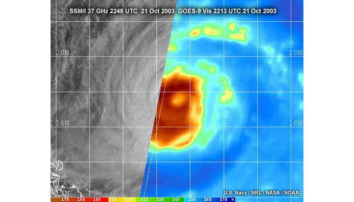
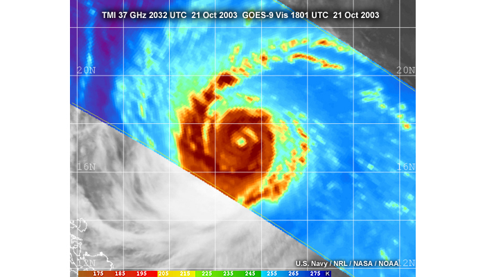
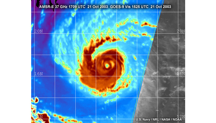
Images from AMSR-E, aboard the Aqua satellite, can give us a preview of CMIS 37 GHz images. First, look at the SSM/I image, then the improvement with TMI, and finally AMSR-E. The CMIS sensor will have the 37 GHz channel at a much higher resolution than the current SSM/I, producing superior images.
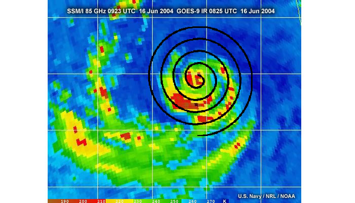
Here’s another example of the benefits of high resolution
at 85 GHz. Earlier we took a quick look at Super Typhoon Dianmu in the Western
Pacific. Can you find the center in this SSM/I 85 GHz image of the storm?
Answer: You can make a reasonable guess at the center following the curvature
of the rainbands, but you cannot see an eye. But does this mean it does not
have one or just that the spatial resolution of the SSM/I is not sufficient
to see it?
7.7 Comparing SSM/I and TMI Images of Dainmu
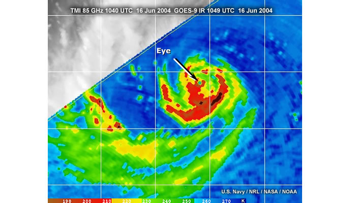
From the relatively coarse resolution of the SSM/I image, the eye is not apparent. However, because of a smaller footprint size, the TMI image from about the same time does show the tiny eye. All other things being equal, higher resolution gives you a better chance of seeing important detail.
Advantages:
Limitations
Advantages:
Limitations:
8.0 Concentric Eyewall Characteristics
8.1 Introduction: Faxasi, Guillermo, and Juliette
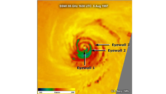
Passive microwave sensors are starting to give us insights into the most powerful hurricanes and typhoons. For example, some tropical cyclones form not just one central eyewall, but sometimes two and even three! Tropical cyclones with multiple eyewalls, as shown here, are very intense and shows Hurricane Guillermo, a relatively small storm.
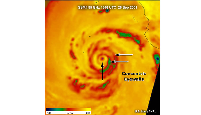
By contrast, Hurricane Juliette from the Eastern Pacific is very large. Near the time of the imaging of Juliette, a reconnaissance aircraft identified three concentric eye walls.
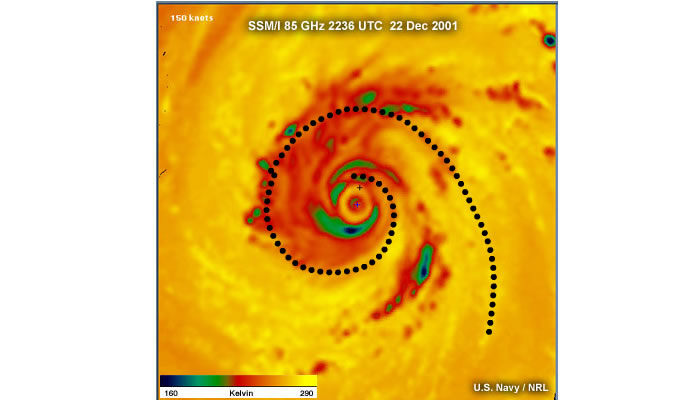
Another Eastern Pacific TS, Faxai has a huge low-level circulation.
8.2 Concentric Eyewall Evolution Modes: Typhoon Saomai
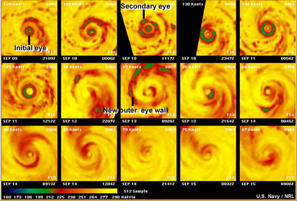
A time-series of SSM/I 85 GHz images over six days shows precipitation bands in green and red, and the sea surface in yellow. At the start of this September 2000 sequence, Typhoon Saomai in the western Pacific had a very small eye, but shortly thereafter developed a secondary outer rainband. The outer rainband completely encircled the small inner eye, cutting off the influx of moisture and energy to the inner eye and eventually causing it to collapse and disappear. An even larger diameter eyewall then formed, apparently starting the process all over again.
8.3 Concentric Eyewall Evolution Example: Super Typhoon Winnie
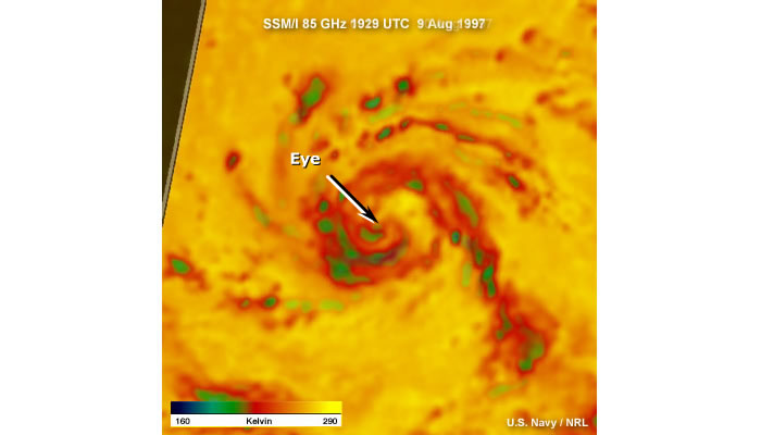
This is an animation of SSM/I 85 GHz views of Super Typhoon Winnie in the western Pacific. First, a small eye develops over a series of images.
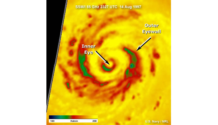
This eye then evolves into a pattern of concentric bands. Gaps in the coverage prevent us from seeing every stage in the transformation. However, we can see snapshots representing profound changes in storm structure that can not be observed by infrared or visible images.
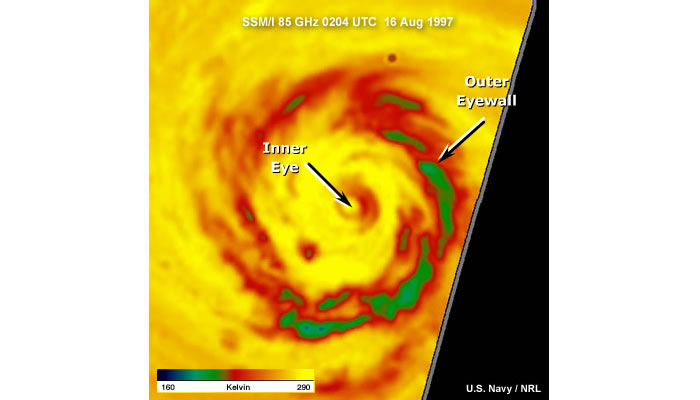
Finally, a very large outer eyewall appears. Note how the small inner eye maintains its structure long after the outer eye defines the dominant circulation. When a storm has well-delineated double eyewalls like this one, the surface winds will most likely also show a double wind maximum underneath the eyewalls. In general, the eyewall with the stronger circulation and vertical motion will also have the higher winds. This will shift depending on the stage of the transition between the smaller inner eye and the larger outer eye.
It can be hard to monitor the evolution of a tropical cyclone when using sequences of passive microwave images from polar-orbiting satellites. The gaps in time are disconcerting, and if you loop the relatively few images that are available, the resulting movie is anything but smooth. Large gaps in time can also make it extremely difficult to infer correct storm motion and intensity changes.
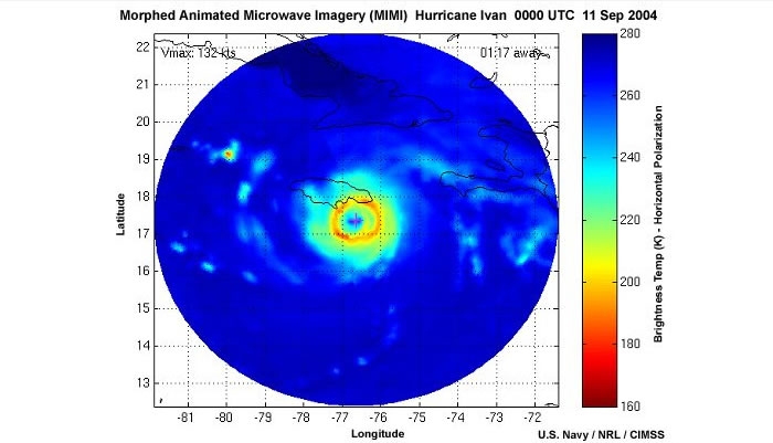
The Cooperative Institute for Meteorological Satellite Studies (CIMSS) has an experimental solution that may help mitigate this problem. The approach is called morphing, a special effect used in movies to produce a smooth transformation from one shape to another. In meteorology, morphing can create images for time intervals without data, for example, during gaps between polar-orbiting satellite overpasses. For this application, simulated scenes are generated for times between successive passive microwave imagery using technique that blends interpolation and advection of the original data. A key assumption for this technique is that the radial wind speed (taken from estimated tropical cyclone winds) is constant during the morphing process.
The result is a series of images now only 15 minutes apart. This is about the frequency of geostationary images. And in fact, the resulting loop looks very much like it was produced from a geostationary satellite! Satellite meteorologists look forward to the day when passive microwave imagers are launched onboard geostationary satellites. But until that time, loops like this one give us a futuristic preview of such a near-realtime capability.Hurricane Ivan shown here was apparently destined to make a direct hit on Jamaica. Look however how the stormtakes a left turn just before the anticipated landfall. The storm was still devastating, but not nearly to the degree had it continued on its more northerly track. This morphed sequence captures this change beautifully. Look at the concentric rain bands that evolve over time. This technique may soon be part of the operational forecaster's toolkit if testing is successful.
Overview
Passive Microwave Sensors
Scan Strategies
Characteristics of Microwave Imagery
At 85-91 GHz:
At 37 GHz:
Tropical Cyclone Characteristics and Interpretation Strategies
Glackin, D.L., J.D. Cunningham, and C.S. Nelson, 2004: Earth remote sensing with NPOESS: instruments and environmental data products. Proc. Sensors, Systems, and Next-Generation Satellites VII. SPIE, 5234, 123-131.
Hawkins, J.D., T.F., J. Turk, C. Sampson, and J. Kent, 2001: Realtime internet distribution of satellite products for tropical cyclone reconnaissance. Bull. Amer. Meteor. Soc., 82, 567-578.
Jones, D., 2004: NPOESS: The next generation system, Earth Observation Magazine, 13, 4-11.
Kidder, S. Q., M. D. Goldberg, R. M. Zehr, M. DeMaria, J. F. W. Purdom, C. S. Velden, N. C. Grody, and S. J. Kusselson, 2000. Satellite analysis of tropical cyclones using the Advanced Microwave Sounding Unit (AMSU). Bull. Amer. Meteor. Soc., 81, 1241–1259.
Lee, T.F., F.J. Turk, J. Hawkins, and K. Richardson, 2002. Interpretation of TRMM TMI images of tropical cyclones. Earth Interactions, 6, paper 3.
Wimmers, A. and C. Veldon, 2004: Morphed anImated Microwave Imagery (MIMI).